Well near a partially penetrating river with leaky bed - comparison with exact solution of Hunt (1999)

Consider flow to a well near a river with a leaky bed. The well is located at \((x,y)=(d, 0)\) and starts pumping at a discharge \(Q\) at time \(t=0\). The river is infinitely long and runs along \(x=0\). The head in the river is fixed (i.e., the drawdown in the river is zero). The width of the river is \(b\) and the resistance of the streambed is \(c\). The width of the river is neglected in the model but taken into account when computing the riverbed conductance.

import matplotlib.pyplot as plt
import numpy as np
from scipy.integrate import quad
from scipy.special import exp1

import timflow.transient as tft

plt.rcParams["figure.figsize"] = (6, 4)

# parameters
k = 10  # hydraulic conductivity, m/d
H = 10  # thickness of aquifer, m
S = 0.1  # phreatic storage, -
c = 5  # streambed resistance, d
b = 5  # stream width, m
d = 100  # distance of well from river, m
Q = 500  # well discharge, m^3/d
# computed parameters
T = k * H
C = b / c  # riverbed conductance, = lambda in Hunt (1999)

The exact solution is given in Hunt (1999), Equation 30.

def func(theta, x, y, t):
    rv = np.exp(-theta) * exp1(
        ((d + np.abs(x) + 2 * T * theta / C) ** 2 + y**2) / (4 * T * t / S)
    )
    return rv


def hunt(x, y, t):
    part1 = exp1(((d - x) ** 2 + y**2) / (4 * T * t / S))
    part2 = quad(func, 0, np.inf, args=(x, y, t))[0]
    return -Q / (4 * np.pi * T) * (part1 - part2)


huntvec = np.vectorize(hunt)

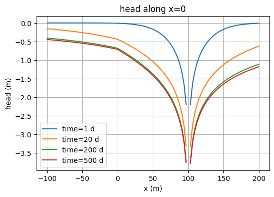
for t in [1, 20, 200, 500]:
    nx = 100
    x = np.linspace(-d, 2 * d, nx)
    y = np.zeros(nx)
    h = huntvec(x, y, t)
    plt.plot(x, h, label=f"time={t} d")
plt.legend()
plt.xlabel("x (m)")
plt.ylabel("head (m)")
plt.title("head along x=0")
plt.grid()

Timflow model

ml = tft.ModelMaq(kaq=k, z=[0, -10], Saq=S, phreatictop=True, tmin=1, tmax=1000)
w = tft.Well(ml, d, 0, tsandQ=[(0, Q)])
yls = np.hstack(
    (
        np.linspace(-1000, -200, 10),
        np.linspace(-200, 200, 10)[1:],
        np.linspace(200, 1000, 10)[1:],
    )
)
xls = np.zeros(len(yls))
xy = np.array([xls, yls]).T
riv = tft.RiverString(ml, xy=xy, tsandh="fixed", res=c, wh=b)
ml.solve()

self.neq  28
solution complete

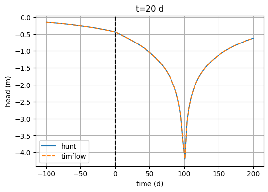
Comparison

x = np.linspace(-100, 200, 101)
y = np.zeros(101)
t = 20
hhunt = huntvec(x, y, t)
plt.plot(x, hhunt, label="hunt")
htim = ml.headalongline(x, y, t)
plt.plot(x, htim[0, 0], "--", label="timflow")
plt.legend()
plt.xlabel("time (d)")
plt.ylabel("head (m)")
plt.title(f"t={t} d")
plt.axvline(0, color="k", ls="--")
plt.grid()

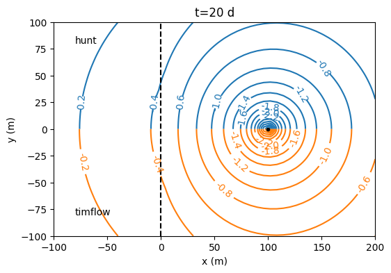
x, y = np.meshgrid(np.linspace(-100, 200, 50), np.linspace(0, 100, 50))
t = 20
h = huntvec(x, y, t)
plt.subplot(111, aspect=1)
cs = plt.contour(x, y, h, levels=np.arange(-4, 0, 0.2), colors="C0")
plt.clabel(cs, fmt="%1.1f")
x, y = np.linspace(-100, 200, 50), np.linspace(-100, 0, 50)
h = ml.headgrid(x, y, t).squeeze()
cs = plt.contour(x, y, h, levels=np.arange(-4, 0, 0.2), colors="C1")
plt.clabel(cs, fmt="%1.1f")
plt.axvline(0, color="k", ls="--")
plt.text(-80, 80, "hunt")
plt.text(-80, -80, "timflow")
plt.title(f"t={t} d")
plt.xlabel("x (m)")
plt.ylabel("y (m)")
plt.plot(d, 0, "k.");

Reference

Hunt, B., 1999. Unsteady stream depletion from ground water pumping. Groundwater, 37(1), pp.98-102, https://doi.org/10.1111/j.1745-6584.1999.tb00962.x