2. Slug Test for Confined Aquifer - Multi-well

Import packages

import matplotlib.pyplot as plt
import numpy as np
import pandas as pd

import timflow.transient as tft

plt.rcParams["figure.figsize"] = [5, 3]

Introduction and Conceptual Model

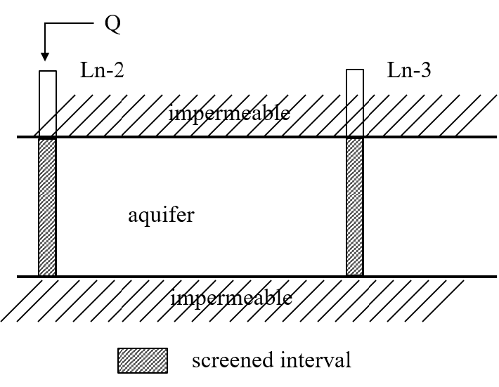
A well (Ln-2) fully penetrates a sandy confined aquifer of 6.1 m thickness. Additionally, a fully penetrating observation well (Ln-3) is located 6.45 m away from the test well. The slug displacement is 2.798 m. Head change was recorded at the slug well and the observation well. The well and casing radii of the slug well are 0.102 and 0.051 m, respectively. For the observation well, they are 0.071 and 0.025 m, respectively.

Load data

data1 = np.loadtxt("data/ln-2.txt")
t1 = data1[:, 0] / 60 / 60 / 24  # convert time from seconds to days
h1 = data1[:, 1]

data2 = np.loadtxt("data/ln-3.txt")
t2 = data2[:, 0] / 60 / 60 / 24
h2 = data2[:, 1]

Parameters and model

# known parameters
H0 = 2.798  # initial displacement, m
b = 6.1  # aquifer thickness, m
rw1 = 0.102  # well radius of Ln-2 Well, m
rw2 = 0.071  # well radius of observation Ln-3 Well, m
rc1 = 0.051  # casing radius of Ln-2 Well, m
r = 6.45  # distance from observation well to test well, m

Converting slug displacement into volume

Q = np.pi * rc1**2 * H0
print(f"Slug: {Q:.5f} m^3")

Slug: 0.02286 m^3

ml = tft.ModelMaq(kaq=10, z=[0, -b], Saq=1e-4, tmin=1e-5, tmax=0.01)
w = tft.Well(ml, xw=0, yw=0, rw=rw1, rc=rc1, tsandQ=[(0, -Q)], layers=0, wbstype="slug")
ml.solve()

self.neq  1
solution complete

Estimate aquifer parameters

The hydraulic conductivity and specific storage are calibrated.

# unknown parameters: kaq, Saq
cal = tft.Calibrate(ml)
cal.set_parameter(name="kaq", layers=0, initial=10)
cal.set_parameter(name="Saq", layers=0, initial=1e-4)
cal.seriesinwell(name="Ln-2", element=w, t=t1, h=h1)
cal.series(name="Ln-3", x=r, y=0, layer=0, t=t2, h=h2)
cal.fit()

...................................
Fit succeeded.

display(cal.parameters.loc[:, ["optimal"]])
print(f"RMSE: {cal.rmse():.3f} m")

	optimal
kaq_0_0	1.166113
Saq_0_0	0.000009

RMSE: 0.010 m

hm1 = w.headinside(t1)
hm2 = ml.head(r, 0, t2, layers=0)
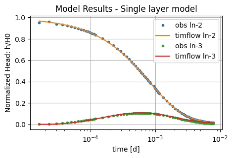
plt.semilogx(t1, h1 / H0, ".", label="obs ln-2")
plt.semilogx(t1, hm1[0] / H0, label="timflow ln-2")
plt.semilogx(t2, h2 / H0, ".", label="obs ln-3")
plt.semilogx(t2, hm2[0] / H0, label="timflow ln-3")
plt.xlabel("time [d]")
plt.ylabel("Normalized Head: h/H0")
plt.title("Model Results - Single layer model")
plt.legend()
plt.grid()

Comparison of results

The values in timflow are compared with the KGS analytical model (Hyder et al. 1994) implemented in AQTESOLV (Duffield, 2007), and to the MLU model (Hemker & Post, 2014). The parameters of timflowand AQTESOLV are very similar. MLU differs a bit, this is likely due to the added skin resistance (skin factor of 2.42).

Show code cell source

Hide code cell source

t = pd.DataFrame(
    columns=["k [m/d]", "Ss [1/m]", "RMSE [m]"],
    index=["timflow", "AQTESOLV", "MLU"],
)

t.loc["timflow"] = np.append(cal.parameters["optimal"].values, cal.rmse())
t.loc["AQTESOLV"] = [1.166, 9.369e-06, "-"]
t.loc["MLU"] = [1.311, 8.197e-06, "-"]

t_formatted = t.style.format(
    {
        "k [m/d]": "{:.2f}",
        "Ss [1/m]": "{:.2e}",
        "RMSE [m]": lambda x: "-" if x == "-" else f"{float(x):.3f}",
    }
)
t_formatted

	k [m/d]	Ss [1/m]	RMSE [m]
timflow	1.17	9.38e-06	0.010
AQTESOLV	1.17	9.37e-06	-
MLU	1.31	8.20e-06	-

References

• Butler Jr., J.J. (1998), The Design, Performance, and Analysis of Slug Tests, Lewis Publishers, Boca Raton, Florida, 252p.

• Hemker, K. and Post V. (2014) MLU for Windows: well flow modeling in multilayer aquifer systems; MLU User’s guide. https://eur03.safelinks.protection.outlook.com/?url=https%3A%2F%2Fmicrofem.com%2Fdownload%2Fmlu-user.pdf&data=05%7C02%7CMark.Bakker%40tudelft.nl%7Cad7f16364d2d4fd55dbf08de73832eaa%7C096e524d692940308cd38ab42de0887b%7C0%7C0%7C639075204580287861%7CUnknown%7CTWFpbGZsb3d8eyJFbXB0eU1hcGkiOnRydWUsIlYiOiIwLjAuMDAwMCIsIlAiOiJXaW4zMiIsIkFOIjoiTWFpbCIsIldUIjoyfQ%3D%3D%7C0%7C%7C%7C&sdata=OBoe8seXZUfoat89Dfr4g6lF%2Bn1FdtXqtp%2F18BMXCn0%3D&reserved=0

• Duffield, G.M. (2007), AQTESOLV for Windows Version 4.5 User’s Guide, HydroSOLVE, Inc., Reston, VA.

• Hyder, Z., Butler Jr, J.J., McElwee, C.D. and Liu, W. (1994), Slug tests in partially penetrating wells, Water Resources Research 30, 2945–2957.