1. Confined Aquifer Test - Oude Korendijk#
Import packages#
import matplotlib.pyplot as plt
import numpy as np
import pandas as pd

import timflow.transient as tft

plt.rcParams["figure.figsize"] = (5, 3)  # default figure size
Introduction and Conceptual Model#
In this example, we will use the pumping test data from Oude Korendijk (Kruseman et al. 1970).
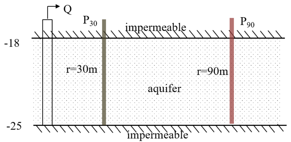
Oude Korendijk is a polder area South of Rotterdam, the Netherlands. The stratigraphy can be summarized by:
the first 18 m consist of almost impermeable material,
the next 7 m is succession of coarse gravel and sands, which are considered as the aquifer layer,
a layer of fine sands and clayey sediments that are deemed impermeable.
The well screens the whole thickness of the confined aquifer. Drawdowns were measured in two piezometers located at distances of 30 m and 90 m from the well. The pumping well discharge was constant at 788 m\(^3\)/d for almost 14 hours. The objective of the pumping test was to estimate the hydraulic conductivity and the specific storage of the aquifer layer.
Load data#
# time and drawdown of piezometer 30m away from pumping well
data1 = np.loadtxt("data/piezometer_h30.txt", skiprows=1)
to1 = data1[:, 0] / 60 / 24  # convert min to days
ho1 = data1[:, 1]
ro1 = 30
# time and drawdown of piezometer 90m away from pumping well
data2 = np.loadtxt("data/piezometer_h90.txt", skiprows=1)
to2 = data2[:, 0] / 60 / 24  # convert min to days
ho2 = data2[:, 1]
ro2 = 90
Parameters and model#
# known parameters
H = 7  # aquifer thickness in meters, m
zt = -18  # top boundary of aquifer, m
zb = zt - H  # bottom boundary of aquifer, m
Q = 788  # constant discharge, m3/d
# timflow model
ml = tft.ModelMaq(kaq=60, z=[zt, zb], Saq=1e-4, tmin=1e-5, tmax=1)
w = tft.Well(model=ml, xw=0, yw=0, rw=0.2, tsandQ=[(0, Q)], layers=0)
ml.solve()
self.neq  1
solution complete
Estimate aquifer parameters#
The aquifer parameters are estimated using head observations at both piezometers.
# unknown parameters: kaq, Saq
cal = tft.Calibrate(ml)
cal.set_parameter(name="kaq", initial=10, layers=0)
cal.set_parameter(name="Saq", initial=1e-4, layers=0)
cal.series(name="obs1", x=ro1, y=0, t=to1, h=ho1, layer=0)  # Adding well 1
cal.series(name="obs2", x=ro2, y=0, t=to2, h=ho2, layer=0)  # Adding well 2
cal.fit(report=False)
.........................
...
Fit succeeded.
display(cal.parameters.loc[:, ["optimal"]])
print(f"RMSE: {cal.rmse():.3f} m")
| optimal | |
|---|---|
| kaq_0_0 | 66.088700 |
| Saq_0_0 | 0.000025 |
RMSE: 0.050 m
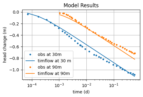
hm1 = ml.head(ro1, 0, to1)
hm2 = ml.head(ro2, 0, to2)
plt.semilogx(to1, ho1, "C0.", label="obs at 30m")
plt.semilogx(to1, hm1[0], "C0", label="timflow at 30 m")
plt.semilogx(to2, ho2, "C1.", label="obs at 90m")
plt.semilogx(to2, hm2[0], "C1", label="timflow at 90m")
plt.title("Model Results")
plt.xlabel("time (d)")
plt.ylabel("head change (m)")
plt.legend()
plt.grid()
Comparison of results#
The performance of timflow was compared with MLU (Hemker & Post, 2014), and Kruseman and de Ridder (1970), here abbreviated to K&dR.
MLU included, compared to timflow, three observation wells in the calibration, located at 30, 90, and 215 m from the pumping well. The fit remains poor for the observations at 215 m, which explains the relatively large RMSE. The late-time drawdowns increase more slowly than the computed Theis drawdowns, which is likely caused by leakage (Kruseman and de Ridder, 1970; Hemker & Post, 2014).
Since timflow only includes the first two observation wells (30 and 90 m), the fit to the data is better. However, the estimated parameters are quite similar to those obtained with MLU, while the solution reported by K&dR shows differences.
| k [m/d] | Ss [1/m] | RMSE [m] | |
|---|---|---|---|
| timflow | 66.09 | 2.54e-05 | 0.050 |
| MLU | 63.51 | 3.58e-05 | 0.833 |
| K&dR | 55.71 | 1.70e-04 | 1.293 |
References#
Bakker, M. (2013), Semi-analytic modeling of transient multi-layer flow with TTim, Hydrogeol J 21, 935–943, https://doi.org/10.1007/s10040-013-0975-2
Duffield, G.M. (2007), AQTESOLV for Windows Version 4.5 User’s Guide, HydroSOLVE, Inc., Reston, VA.
Hemker, K. en Post V. (2014) MLU for Windows: well flow modeling in multilayer aquifer systems; MLU User’s guide. https://eur03.safelinks.protection.outlook.com/?url=https%3A%2F%2Fmicrofem.com%2Fdownload%2Fmlu-user.pdf&data=05%7C02%7CMark.Bakker%40tudelft.nl%7Cad7f16364d2d4fd55dbf08de73832eaa%7C096e524d692940308cd38ab42de0887b%7C0%7C0%7C639075204580287861%7CUnknown%7CTWFpbGZsb3d8eyJFbXB0eU1hcGkiOnRydWUsIlYiOiIwLjAuMDAwMCIsIlAiOiJXaW4zMiIsIkFOIjoiTWFpbCIsIldUIjoyfQ%3D%3D%7C0%7C%7C%7C&sdata=OBoe8seXZUfoat89Dfr4g6lF%2Bn1FdtXqtp%2F18BMXCn0%3D&reserved=0
Kruseman, G.P., De Ridder, N.A. and Verweij, J.M. (1970), Analysis and evaluationof pumping test data, volume 11, International institute for land reclamation and improvement The Netherlands.