Synthetic Pumping Test - Calibration

import matplotlib.pyplot as plt
import numpy as np

from timflow import transient as tft

plt.rcParams["figure.figsize"] = (6, 4)

Use observation times from Oude Korendijk

drawdown = np.loadtxt("../04pumpingtests/data/oudekorendijk_h30.dat")

tobs = drawdown[:, 0] / 60 / 24
robs = 30
Q = 788

Generate data

ml = tft.ModelMaq(kaq=60, z=(-18, -25), Saq=1e-4, tmin=1e-5, tmax=1)
w = tft.Well(ml, xw=0, yw=0, rw=0.1, tsandQ=[(0, 788)], layers=0)
ml.solve()
rnd = np.random.default_rng(2)
hobs = ml.head(robs, 0, tobs)[0] + 0.05 * rnd.random(len(tobs))

self.neq  1
solution complete

See if timflow.transient can find aquifer parameters back

cal = tft.Calibrate(ml)
cal.set_parameter(name="kaq", layers=0, initial=100)
cal.set_parameter(name="Saq", layers=0, initial=1e-3)
cal.series(name="obs1", x=robs, y=0, layer=0, t=tobs, h=hobs)
cal.fit()

............................
........
Fit succeeded.

cal.parameters

	layers	optimal	std	perc_std	pmin	pmax	initial	inhoms	parray
kaq_0_0	0	59.871358	0.670180	1.119366	-inf	inf	100.000	None	[[59.87135844623144]]
Saq_0_0	0	0.000121	0.000004	3.633645	-inf	inf	0.001	None	[[0.00012118958795889718]]

print("rmse:", cal.rmse())

rmse: 0.014201293762177191

hm = ml.head(robs, 0, tobs, 0)
plt.semilogx(tobs, hobs, ".k")
plt.semilogx(tobs, hm[0], "r");

print("correlation matrix")
print(cal.fitresult.covar)

correlation matrix
[[ 4.49140659e-01 -2.49689444e-06]
 [-2.49689444e-06  1.93916877e-11]]

Fit with scipy.least_squares (not recommended)

cal = tft.Calibrate(ml)
cal.set_parameter(name="kaq", layers=0, initial=100)
cal.set_parameter(name="Saq", layers=0, initial=1e-3)
cal.series(name="obs1", x=robs, y=0, layer=0, t=tobs, h=hobs)
cal.fit_least_squares(report=True)

..........................
..
............
         layers    optimal       std  perc_std  pmin  pmax  initial inhoms  \
kaq_0_0       0  59.870813  0.660194  1.102698  -inf   inf  100.000   None   
Saq_0_0       0   0.000121  0.000004  3.590897  -inf   inf    0.001   None   

                             parray  
kaq_0_0      [[59.870812856482374]]  
Saq_0_0  [[0.00012119422744882299]]  
[6.60194017e-01 4.35195992e-06]
[[ 4.35856140e-01 -2.42941594e-06]
 [-2.42941594e-06  1.89395552e-11]]
[[ 1.        -0.8455619]
 [-0.8455619  1.       ]]

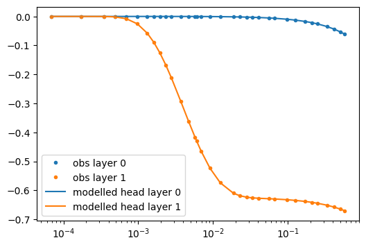
Calibrate parameters in multiple layers

Example showing how parameters can be optimized when multiple layers share the same parameter value.

ml = tft.ModelMaq(
    kaq=[10.0, 10.0],
    z=(-10, -16, -18, -25),
    c=[10.0],
    Saq=[0.1, 1e-4],
    tmin=1e-5,
    tmax=1,
)
w = tft.Well(ml, xw=0, yw=0, rw=0.1, tsandQ=[(0, 788)], layers=1)
ml.solve()
hobs0 = ml.head(robs, 0, tobs, layers=[0])[0]
hobs1 = ml.head(robs, 0, tobs, layers=[1])[0]

self.neq  1
solution complete

cal.parameters

	layers	optimal	std	perc_std	pmin	pmax	initial	inhoms	parray
kaq_0_0	0	59.870813	0.660194	1.102698	-inf	inf	100.000	None	[[59.870812856482374]]
Saq_0_0	0	0.000121	0.000004	3.590897	-inf	inf	0.001	None	[[0.00012119422744882299]]

cal = tft.Calibrate(ml)
cal.set_parameter(
    name="kaq", layers=[0, 1], initial=20.0, pmin=0.0, pmax=30.0
)  # layers 0 and 1 have the same k-value
cal.set_parameter(name="Saq", layers=0, initial=1e-3, pmin=1e-5, pmax=0.2)
cal.set_parameter(name="Saq", layers=1, initial=1e-3, pmin=1e-5, pmax=0.2)
cal.set_parameter(name="c", layers=1, initial=1.0, pmin=0.1, pmax=200.0)
cal.series(name="obs0", x=robs, y=0, layer=0, t=tobs, h=hobs0)
cal.series(name="obs1", x=robs, y=0, layer=1, t=tobs, h=hobs1)
cal.fit(report=False)
display(cal.parameters)

......
..
...........
..
..
......
..
...........
..
..
......
..
...........
..
..
......
..
...........
..
..
......
..
...........
..
..
......
..
...........
..
..
......
..
.
Fit succeeded.

	layers	optimal	std	perc_std	pmin	pmax	initial	inhoms	parray
kaq_0_1	[0, 1]	9.997946	5.591961e-04	0.005593	0.00000	30.0	20.000	None	[[9.997945851630666, 9.997945851630666]]
Saq_0_0	0	0.100017	4.573867e-07	0.000457	0.00001	0.2	0.001	None	[[0.10001677499704055]]
Saq_1_1	1	0.000100	2.007608e-09	0.002008	0.00001	0.2	0.001	None	[[9.999147652238387e-05]]
c_1_1	1	9.999392	1.692171e-04	0.001692	0.10000	200.0	1.000	None	[[9.999392198555688]]

plt.semilogx(tobs, hobs0, ".C0", label="obs layer 0")
plt.semilogx(tobs, hobs1, ".C1", label="obs layer 1")

hm = ml.head(robs, 0, tobs)
plt.semilogx(tobs, hm[0], "C0", label="modelled head layer 0")
plt.semilogx(tobs, hm[1], "C1", label="modelled head layer 1")

plt.legend(loc="best");

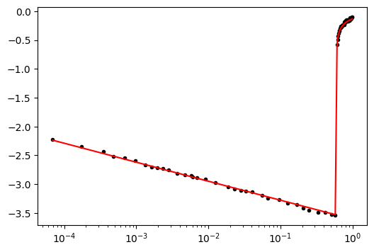
Generate data for head measured in well

tobs2 = np.hstack((tobs, np.arange(0.61, 1, 0.01)))

ml = tft.ModelMaq(kaq=60, z=(-18, -25), Saq=1e-4, tmin=1e-5, tmax=1)
w = tft.Well(ml, xw=0, yw=0, rw=0.3, res=0.02, tsandQ=[(0, 788), (0.6, 0)], layers=0)
ml.solve()
rnd = np.random.default_rng(2)
hobs2 = w.headinside(tobs2)[0] + 0.05 * rnd.random(len(tobs2))

self.neq  1
solution complete

cal = tft.Calibrate(ml)
cal.set_parameter(name="kaq", layers=0, initial=100)
cal.set_parameter(name="Saq", layers=0, initial=1e-3)
cal.set_parameter_by_reference(name="res", parameter=w.res[:], initial=0.05)
cal.seriesinwell(name="obs1", element=w, t=tobs2, h=hobs2)
cal.fit()

..........................
..
.........................
..
..........................
..
..........................
.
...........................
.
..........................
..
..........................
..
.........................
..
..........................
..
.........................
...
........................
....
........................
...
.........................
...
.........................
...
.................
Fit succeeded.

hm = w.headinside(tobs2)
plt.semilogx(tobs2, hobs2, ".k")
plt.semilogx(tobs2, hm[0], "r");