3. Confined Aquifer Test - Sioux Flats

Import packages

import matplotlib.pyplot as plt
import numpy as np
import pandas as pd

import timflow.transient as tft

plt.rcParams["figure.figsize"] = (5, 3)  # default figure size

Introduction and Conceptual Model

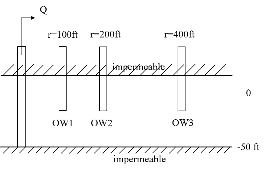
This example is a pumping test done in Sioux Flats, South Dakota, USA. The data comes from the AQTESOLV documentation (Duffield, 2007).

The aquifer is 50 ft thick and is bounded by impermeable layers. The test was conducted for 2045 minutes (~34 hours), with a constant pumping rate of 2.7 ft\(^3\)/s. Drawdown data has been collected at three piezometers located 100, 200 and 400 ft away, respectively. The well radius is 0.5 ft.

Load data

# time and drawdown of piezometer 100ft away from pumping well
data1 = np.loadtxt("data/sioux100.txt")
t1 = data1[:, 0]
h1 = data1[:, 1]

# time and drawdown of piezometer 200ft away from pumping well
data2 = np.loadtxt("data/sioux200.txt")
t2 = data2[:, 0]
h2 = data2[:, 1]

# time and drawdown of piezometer 300ft away from pumping well
data3 = np.loadtxt("data/sioux400.txt")
t3 = data3[:, 0]
h3 = data3[:, 1]

Parameters and model

# known parameters
Q = (
    (2.7 * 0.3048**3) * 60 * 60 * 24
)  # constant discharge in m^3/d (2.7 ft^3/s = 6605.754 m^3/d)
b = 50 * 0.3048  # aquifer thickness in m (50 ft = 15.24 m)
rw = 0.5 * 0.3048  # well radius in m (0.5 ft = 0.1524 m)
r1 = 100 * 0.3048  # distance between obs1 to pumping well (100 ft = 30.48 m)
r2 = 200 * 0.3048  # distance between obs2 to pumping well (200 ft = 60.96 m)
r3 = 400 * 0.3048  # distance between obs3 to pumping well (400 ft = 121.92 m)

# timflow model
ml = tft.ModelMaq(kaq=10, z=[0, -b], Saq=0.001, tmin=0.001, tmax=10, topboundary="conf")
w = tft.Well(ml, xw=0, yw=0, rw=rw, tsandQ=[(0, Q)], layers=0)
ml.solve()

self.neq  1
solution complete

Estimate aquifer parameters

# unknown parameters: k, Saq
cal = tft.Calibrate(ml)
cal.set_parameter(name="kaq", initial=10, layers=0)
cal.set_parameter(name="Saq", initial=1e-4, layers=0)
cal.series(name="obs1", x=r1, y=0, t=t1, h=h1, layer=0)  # Adding well 1
cal.series(name="obs2", x=r2, y=0, t=t2, h=h2, layer=0)  # Adding well 2
cal.series(name="obs3", x=r3, y=0, t=t3, h=h3, layer=0)  # Adding well 3
cal.fit(report=False)

...............................
............
Fit succeeded.

display(cal.parameters.loc[:, ["optimal"]])
print(f"RMSE: {cal.rmse():.3f} m")

	optimal
kaq_0_0	282.794933
Saq_0_0	0.004209

RMSE: 0.004 m

hm1 = ml.head(r1, 0, t1)
hm2 = ml.head(r2, 0, t2)
hm3 = ml.head(r3, 0, t3)
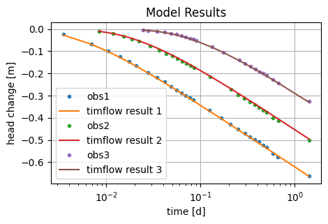
plt.semilogx(t1, h1, ".", label="obs1")
plt.semilogx(t1, hm1[0], label="timflow result 1")
plt.semilogx(t2, h2, ".", label="obs2")
plt.semilogx(t2, hm2[0], label="timflow result 2")
plt.semilogx(t3, h3, ".", label="obs3")
plt.semilogx(t3, hm3[0], label="timflow result 3")
plt.title("Model Results")
plt.xlabel("time [d]")
plt.ylabel("head change [m]")
plt.legend()
plt.grid()

Comparison of results

The performance of timflow is compared to the results based on Theis’ analytical solution (Theis, 1935), implemented in the software AQTESOLV (Duffield, 2007).

timflow achieved similar results as AQTESOLV.

Show code cell source

Hide code cell source

t = pd.DataFrame(
    columns=["k [m/d]", "Ss [1/m]", "RMSE [m]"], index=["timflow", "AQTESOLV"]
)

t.loc["timflow"] = np.append(cal.parameters["optimal"].values, cal.rmse())
t.loc["AQTESOLV"] = [282.659, 4.0355e-03, "-"]

t_formatted = t.style.format(
    {
        "k [m/d]": "{:.2f}",
        "Ss [1/m]": "{:.2e}",
        "RMSE [m]": lambda x: "-" if x == "-" else f"{float(x):.3f}",
    }
)
t_formatted

	k [m/d]	Ss [1/m]	RMSE [m]
timflow	282.79	4.21e-03	0.004
AQTESOLV	282.66	4.04e-03	-

References

• Duffield, G.M. (2007), AQTESOLV for Windows Version 4.5 User’s Guide, HydroSOLVE, Inc., Reston, VA.

• Newville, M., Stensitzki, T., Allen, D.B., Ingargiola, A. (2014), LMFIT: Non Linear Least-Squares Minimization and Curve Fitting for Python, https://dx.doi.org/10.5281/zenodo.11813, https://lmfit.github.io/lmfit-py/intro.html (last access: August,2021).