1.Test for an anisotropic water-table aquifer - Moench Example#
Import packages#
import matplotlib.pyplot as plt
import numpy as np
import pandas as pd

import timflow.transient as tft

plt.rcParams["figure.figsize"] = (5, 3)  # default figure size
Introduction and Conceptual Model#
This test is based on a synthetic example reported by Barlow and Moench (1999), utilizing an analytical solution developed by Moench and Allen (1997) for the transient flow of partially-penetrating wells in unconfined aquifers.
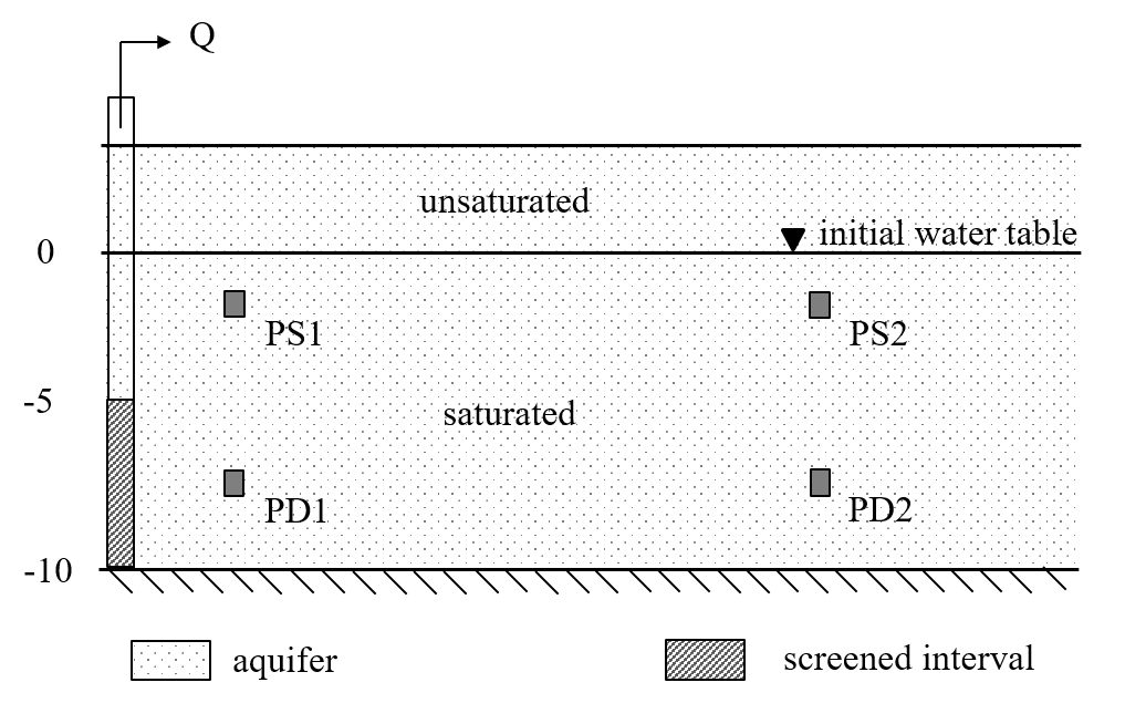
The aquifer is partially saturated with water (10 m water table). A pumping well is screened from 5 to 10 m depth. The well and the well-casing radius is 0.1 m.
Drawdown is recorded at the pumping well and four piezometers located at two different distances and two different depths. Two piezometers, PS1 and PS2, are located at one-meter depth below the water table and 3.16 and 31.6 m distance, respectively. Another two (PD1 and PD2) piezometers are at 7.5 m depth below the water table and the same distances, directly below the previous piezometers. The figure below shows the location of the well and the piezometers
Pumping starts at time t = 0 at a constant rate of 172.8 m3/d. Drawdown is recorded until t = 3 days.
Load data#
The dataset for each well consists of a column with the time data in seconds and drawdown in meters. We are loading it and converting it to days and meters.
data0 = np.loadtxt("data/moench_pumped.txt", skiprows=1)
t0 = data0[:, 0] / 60 / 60 / 24  # convert time from seconds to days
h0 = -data0[:, 1]  # converting drawdown to heads
data1 = np.loadtxt("data/moench_ps1.txt", skiprows=1)
t1 = data1[:, 0] / 60 / 60 / 24  # convert time from seconds to days
h1 = -data1[:, 1]
data2 = np.loadtxt("data/moench_pd1.txt", skiprows=1)
t2 = data2[:, 0] / 60 / 60 / 24  # convert time from seconds to days
h2 = -data2[:, 1]
data3 = np.loadtxt("data/moench_ps2.txt", skiprows=1)
t3 = data3[:, 0] / 60 / 60 / 24  # convert time from seconds to days
h3 = -data3[:, 1]
data4 = np.loadtxt("data/moench_pd2.txt", skiprows=1)
t4 = data4[:, 0] / 60 / 60 / 24  # convert time from seconds to days
h4 = -data4[:, 1]
Parameters and model#
b = 10  # aquifer thickness, m
Q = 172.8  # constant discharge rate, m^3/d
rw = 0.1  # well radius, m
rc = 0.1  # casing radius, m
r1 = 3.16  # distance of closer wells, m
r2 = 31.6  # distance of wells more far away, m
ml = tft.Model3D(
    kaq=1,
    z=[0, -0.1, -2.1, -5.1, -10.1],
    Saq=[0.1, 1e-4, 1e-4, 1e-4],
    kzoverkh=1,
    tmin=1e-5,
    tmax=3,
    phreatictop=True,
)
w = tft.Well(ml, xw=0, yw=0, rw=rw, rc=rc, tsandQ=[(0, Q)], layers=3)
ml.solve()
self.neq  1
solution complete
Estimate aquifer parameters#
cal = tft.Calibrate(ml)
cal.set_parameter(name="kaq", initial=1, layers=[0, 1, 2, 3])
cal.set_parameter(name="Saq", initial=0.2, layers=[0])
cal.set_parameter(name="Saq", initial=1e-4, pmin=0, layers=[1, 2, 3])
cal.set_parameter(name="kzoverkh", initial=0.1, pmin=0, layers=[0, 1, 2, 3])

cal.seriesinwell(name="pumped", element=w, t=t0, h=h0)

cal.series(name="PS1", x=r1, y=0, t=t1, h=h1, layer=1)
cal.series(name="PD1", x=r1, y=0, t=t2, h=h2, layer=3)
cal.series(name="PS2", x=r2, y=0, t=t3, h=h3, layer=1)
cal.series(name="PD2", x=r2, y=0, t=t4, h=h4, layer=3)

cal.fit(report=False)
...............
................
................
................
...
Fit succeeded.
display(cal.parameters.loc[:, ["optimal"]])
print(f"RMSE: {cal.rmse():.3f} m")
| optimal | |
|---|---|
| kaq_0_3 | 9.067661 |
| Saq_0_0 | 0.172878 |
| Saq_1_3 | 0.000039 |
| kzoverkh_0_3 | 0.535049 |
RMSE: 0.010 m
hm0 = ml.head(0, 0, t0, layers=3)[0]
hm1 = ml.head(r1, 0, t1, layers=1)[0]
hm2 = ml.head(r1, 0, t2, layers=3)[0]
hm3 = ml.head(r2, 0, t3, layers=1)[0]
hm4 = ml.head(r2, 0, t4, layers=3)[0]
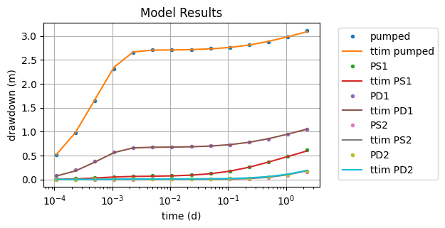
plt.semilogx(t0, -h0, ".", label="pumped")
plt.semilogx(t0, -hm0, label="ttim pumped")
plt.semilogx(t1, -h1, ".", label="PS1")
plt.semilogx(t1, -hm1, label="ttim PS1")
plt.semilogx(t2, -h2, ".", label="PD1")
plt.semilogx(t2, -hm2, label="ttim PD1")
plt.semilogx(t3, -h3, ".", label="PS2")
plt.semilogx(t3, -hm3, label="ttim PS2")
plt.semilogx(t4, -h4, ".", label="PD2")
plt.semilogx(t4, -hm4, label="ttim PD2")
plt.xlabel("time (d)")
plt.ylabel("drawdown (m)")
plt.title("Model Results")
plt.legend(bbox_to_anchor=(1.05, 1))
plt.grid();
Comparison of results#
The performance of timflow is compared with the stimulated results using Moench’s parameters (Barlow and Moench, 1999). The RMSE decreased with the performance of timflow.
| k [m/d] | Sy [-] | Ss [1/m] | kz/kh | RMSE [m] | |
|---|---|---|---|---|---|
| timflow | 9.07 | 0.2 | 3.87e-05 | 0.5 | 0.0104 |
| Moench | 8.64 | 0.2 | 2.00e-05 | 0.5 | 0.0613 |
References#
Barlow, P.M., Moench, A.F., 1999. WTAQ, a computer program for calculating drawdowns and estimating hydraulic properties for confined and water-table aquifers. 99-4225, US Dept. of the Interior, US Geological Survey
Moench, Allen, F., 1997. Flow to a well of finite diameter in a homogeneous, anisotropic water table aquifer. Water Resources Research 34, 2431–2432.