1. Leaky Aquifer Test - Dalem#

Import packages#

import matplotlib.pyplot as plt
import numpy as np
import pandas as pd

import timflow.transient as tft

plt.rcParams["figure.figsize"] = [5, 3]

Introduction and Conceptual Model#

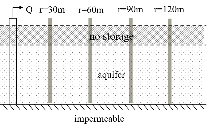
This example is a pumping test from Dalem, the Netherlands (Kruseman and de Ridder, 1970). An aquifer of 37 m thickness is overlain by a semi-confining layer of 8 m thick. Water is pumped from the aquifer and drawdown is recorded at four different piezometers, 30, 60, 90 and 120 m away from the well. The pumping lasted 8 hours in total at a rate of 761 m\(^3\)/d. There is a river 1500 m away from the well. The tide affects both river and well levels. Data was corrected for the tide effect.

Load Data#

# data of observation well 30 m away from pumping well
data1 = np.loadtxt("data/dalem_p30.txt", skiprows=1)
t1 = data1[:, 0]
h1 = data1[:, 1]

# data of observation well 60 m away from pumping well
data2 = np.loadtxt("data/dalem_p60.txt", skiprows=1)
t2 = data2[:, 0]
h2 = data2[:, 1]

# data of observation well 90 m away from pumping well
data3 = np.loadtxt("data/dalem_p90.txt", skiprows=1)
t3 = data3[:, 0]
h3 = data3[:, 1]

# data of observation well 120 m away from pumping well
data4 = np.loadtxt("data/dalem_p120.txt", skiprows=1)
t4 = data4[:, 0]
h4 = data4[:, 1]

Parameters and model#

# known parameters
H = 37  # aquifer thickness in m
zt = -8  # top boundary of aquifer in m
zb = zt - H  # bottom boundary of the aquifer in m
Q = 761  # constant pumping rate in m^3/d
t = 8 / 24  # total pumping time in days (8 hours = 0.34 days)

r1 = 30  # distance from pumping well to observation well 1 in m
r2 = 60  # distance from pumping well to observation well 2 in m
r3 = 90  # distance from pumping well to observation well 3 in m
r4 = 120  # distance from pumping well to observation well 4 in m

The timflow model consists of a single semi-confined aquifer and a pumping well.

# unkonwn parameters: kaq, Saq, c
ml = tft.ModelMaq(
    kaq=10, z=[0, zt, zb], c=500, Saq=1e-4, topboundary="semi", tmin=0.01, tmax=1
)
w = tft.Well(ml, xw=0, yw=0, tsandQ=[(0, Q)])
ml.solve(silent="True")

Estimate aquifer parameters#

The hydraulic condivity and specific storage coefficient of the aquifer are estimated and the resistance of the leaky semi-confining layer.

cal = tft.Calibrate(ml)
cal.set_parameter(name="kaq", initial=10, layers=0)
cal.set_parameter(name="Saq", initial=1e-4, layers=0)
cal.set_parameter(name="c", initial=500, pmin=0, layers=0)

cal.series(name="obs1", x=30, y=0, t=t1, h=h1, layer=0)
cal.series(name="obs2", x=60, y=0, t=t2, h=h2, layer=0)
cal.series(name="obs3", x=90, y=0, t=t3, h=h3, layer=0)
cal.series(name="obs4", x=120, y=0, t=t4, h=h4, layer=0)
cal.fit(report=False)

..........................................
Fit succeeded.

display(cal.parameters.loc[:, ["optimal"]])
print(f"RMSE: {cal.rmse():.5f} m")

	optimal
kaq_0_0	45.331929
Saq_0_0	0.000048
c_0_0	331.165483

RMSE: 0.00592 m

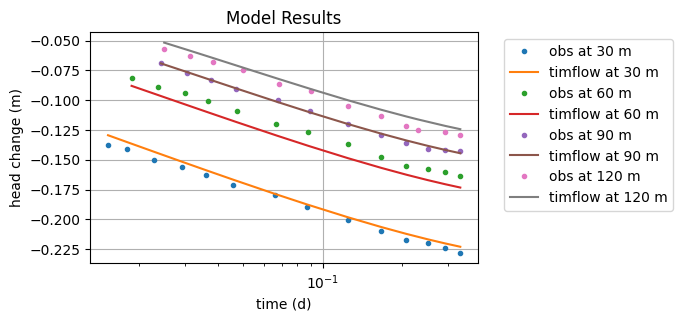
hm_1 = ml.head(r1, 0, t1)
plt.semilogx(t1, h1, ".", label="obs at 30 m")
plt.semilogx(t1, hm_1[0], label="timflow at 30 m")

hm_2 = ml.head(r2, 0, t2)
plt.semilogx(t2, h2, ".", label="obs at 60 m")
plt.semilogx(t2, hm_2[0], label="timflow at 60 m")

hm_3 = ml.head(r3, 0, t3)
plt.semilogx(t3, h3, ".", label="obs at 90 m")
plt.semilogx(t3, hm_3[0], label="timflow at 90 m")

hm_4 = ml.head(r4, 0, t4)
plt.semilogx(t4, h4, ".", label="obs at 120 m")
plt.semilogx(t4, hm_4[0], label="timflow at 120 m")

plt.xlabel("time (d)")
plt.ylabel("head change (m)")
plt.title("Model Results")
plt.legend(bbox_to_anchor=(1.05, 1))
plt.grid();

../../_images/2c22d90711c5485a9a69b413d95e31322ef0c278900883525841f8c44846b296.png

Estimate aquifer parameters using weights#

The head change is smaller in the observation wells that are farther away from the pumping well. It may possibly be expected that the difference between the modeled and measured values is smaller when the total drawdown is smaller. This may be taken into account by giving the measurements weights. In the calibration below, the weight for each observation well is equal to one divided by the maximum absolute head change in that overservation well. It is up to the modeler to decide whether such a weighing is desirable. Note that the root mean squared error (computed without weights) is a bit larger than for the case without the weights, but the increase is small. The fitted values of \(k\) and \(S_s\) are similar to the case without weights, but the resistance \(c\) is quite a bit larger.

cal2 = tft.Calibrate(ml)
cal2.set_parameter(name="kaq", initial=10, layers=0)
cal2.set_parameter(name="Saq", initial=1e-4, layers=0)
cal2.set_parameter(name="c", initial=500, pmin=0, layers=0)

cal2.series(name="obs1", x=30, y=0, t=t1, h=h1, layer=0, weights=1 / np.max(np.abs(h1)))
cal2.series(name="obs2", x=60, y=0, t=t2, h=h2, layer=0, weights=1 / np.max(np.abs(h2)))
cal2.series(name="obs3", x=90, y=0, t=t3, h=h3, layer=0, weights=1 / np.max(np.abs(h3)))
cal2.series(name="obs4", x=120, y=0, t=t4, h=h4, layer=0, weights=1 / np.max(np.abs(h4)))
cal2.fit(report=False)

...............................................
Fit succeeded.

display(cal2.parameters[["optimal"]])
print(f"RMSE: {cal2.rmse(weighted=False):.3f} m")

	optimal
kaq_0_0	48.040548
Saq_0_0	0.000044
c_0_0	539.725730

RMSE: 0.006 m

Comparison of results#

The performance of timflow is compared with other models and with parameter values reported in Kruseman and de Ridder (1970). The published values were obtained by graphical matching to a Hantush type curve (Hantush, 1955). In addition to the timflow results and the literature values, results from AQTESOLV (Duffield, 2007) and MLU (Hemker & Post, 2014) are included for comparison. Both AQTESOLV and MLU were applied to minimize the sum of the squared log-transformed drawdowns. AQTESOLV only fitted the model to the observation well at r = 90 m, whereas the other models were calibrated using data from multiple observation wells.

Overall, all models yield similar estimates of the hydraulic conductivity and specific storage coefficient. The fitted value of the resistance differs. However, the timflow results differ substantially from the MLU and AQTESOLV solutions with respect to aquitard storage and hydraulic resistance.

	k [m/d]	Ss [1/m]	c [d]	RMSE [m]
timflow	45.33	4.76e-05	331	0.0059
timflow weights	48.04	4.36e-05	540	0.0062
AQTESOLV	41.56	4.46e-05	328	0.0382
MLU	45.30	4.86e-05	328	0.0424
Hantush	45.33	4.76e-05	331	0.0059

References#

Bakker, M. (2013), Semi-analytic modeling of transient multi-layer flow with TTim, Hydrogeol J 21, 935–943, https://doi.org/10.1007/s10040-013-0975-2
Duffield, G.M., (2007), AQTESOLV for Windows Version 4.5 User’s Guide, HydroSOLVE, Inc., Reston, VA.
Hemker, K. en Post V. (2014) MLU for Windows: well flow modeling in multilayer aquifer systems; MLU User’s guide. https://eur03.safelinks.protection.outlook.com/?url=https%3A%2F%2Fmicrofem.com%2Fdownload%2Fmlu-user.pdf&data=05%7C02%7CMark.Bakker%40tudelft.nl%7Cad7f16364d2d4fd55dbf08de73832eaa%7C096e524d692940308cd38ab42de0887b%7C0%7C0%7C639075204580287861%7CUnknown%7CTWFpbGZsb3d8eyJFbXB0eU1hcGkiOnRydWUsIlYiOiIwLjAuMDAwMCIsIlAiOiJXaW4zMiIsIkFOIjoiTWFpbCIsIldUIjoyfQ%3D%3D%7C0%7C%7C%7C&sdata=OBoe8seXZUfoat89Dfr4g6lF%2Bn1FdtXqtp%2F18BMXCn0%3D&reserved=0
Kruseman, G.P., De Ridder, N.A. and Verweij, J.M., (1970), Analysis and evaluationof pumping test data, volume 11, International institute for land reclamation and improvement The Netherlands.
Newville, M., Stensitzki, T., Allen, D.B. and Ingargiola, A. (2014), LMFIT: Non Linear Least-Squares Minimization and Curve Fitting for Python, https://dx.doi.org/10.5281/zenodo.11813, https://lmfit.github.io/lmfit-py/intro.html (last access: August,2021).