3. Leaky Aquifer Test - Texas Hill#
Import packages#
import matplotlib.pyplot as plt
import numpy as np
import pandas as pd

import timflow.transient as tft

plt.rcParams["figure.figsize"] = [5, 3]
Introduction and Conceptual Model#
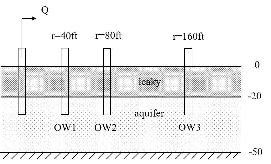
This example concerns a pumping test conducted in the location of Texas Hill and is taken from the AQTESOLV examples (Duffield, 2007). A pumping well is screened in an aquifer located between 20 ft and 70 ft depths. The aquifer is overlain by an aquitard. The formation at the base of the aquifer is considered impermeable.
Three observation wells are located at 40, 80, and 160 ft distance. They are called OW1, OW2, and OW3, respectively. Pumping lasted for 420 minutes at a rate of 4488 gallons per minute.
Load data#
# data of OW1
data1 = np.loadtxt("data/texas40.txt")
t1 = data1[:, 0]  # days
h1 = data1[:, 1]  # meters
r1 = 40 * 0.3048  # distance between obs1 to pumping well in m

# data of OW2
data2 = np.loadtxt("data/texas80.txt")
t2 = data2[:, 0]
h2 = data2[:, 1]
r2 = 80 * 0.3048  # distance between obs2 to pumping well in m

# data of OW3
data3 = np.loadtxt("data/texas160.txt")
t3 = data3[:, 0]
h3 = data3[:, 1]
r3 = 160 * 0.3048  # distance between obs3 to pumping well in m
Parameters and model#
# known parameters
Q = (4488 * 0.00378541) * 60 * 24  # discharge, m^3/d
b1 = 20 * 0.3048  # overlying aquitard thickness, m
b2 = 50 * 0.3048  # aquifer thickness, m
zt = -b1  # top of aquifer, m
zb = -b1 - b2  # bottom of aquifer, m
rw = 0.5 * 0.3048  # well radius, m
The overlying layer is modeld as an aquitard without storage (Sll, the storage parameter, is set to zero in ModelMaq).
ml = tft.ModelMaq(
    kaq=10,
    z=[0, zt, zb],
    Saq=0.001,
    Sll=0,
    c=10,
    tmin=0.001,
    tmax=1,
    topboundary="semi",
)
w = tft.Well(ml, xw=0, yw=0, rw=rw, tsandQ=[(0, Q)], layers=0)
ml.solve()
self.neq  1
solution complete
Estimate aquifer parameters#
The hydraulic parameters of the aquifer (kaq and Saq) and the aquitard (c) are estimated using observations in all three observation wells.
# unknown parameters: kaq, Saq, c
cal = tft.Calibrate(ml)
cal.set_parameter(name="kaq", layers=0, initial=10)
cal.set_parameter(name="Saq", layers=0, initial=1e-4)
cal.set_parameter(name="c", layers=0, initial=100)
cal.series(name="OW1", x=r1, y=0, t=t1, h=h1, layer=0)
cal.series(name="OW2", x=r2, y=0, t=t2, h=h2, layer=0)
cal.series(name="OW3", x=r3, y=0, t=t3, h=h3, layer=0)
cal.fit(report=False)
........................................
..............
Fit succeeded.
display(cal.parameters.loc[:, ["optimal"]])
print(f"RMSE: {cal.rmse():.3f} m")
| optimal | |
|---|---|
| kaq_0_0 | 224.629574 |
| Saq_0_0 | 0.000213 |
| c_0_0 | 43.882999 |
RMSE: 0.060 m
# plot the fitted curves
hm1_1 = ml.head(r1, 0, t1)
hm2_1 = ml.head(r2, 0, t2)
hm3_1 = ml.head(r3, 0, t3)
plt.semilogx(t1, h1, ".", label="OW1")
plt.semilogx(t1, hm1_1[0], label="timflow OW1")
plt.semilogx(t2, h2, ".", label="OW2")
plt.semilogx(t2, hm2_1[0], label="timflow OW2")
plt.semilogx(t3, h3, ".", label="OW3")
plt.semilogx(t3, hm3_1[0], label="timflow OW3")
plt.xlabel("time (d)")
plt.ylabel("head change (m)")
plt.legend(bbox_to_anchor=(1.05, 1))
plt.grid()
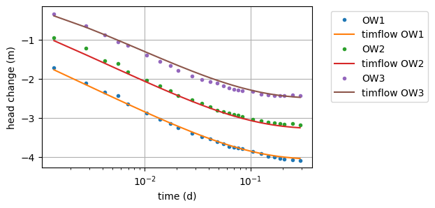
Comparison of Results#
The aquifer response obtained with timflow is compared to the results based on Hantush’s analytical solution (Hantush, 1955), implemented in the software AQTESOLV (Duffield, 2007). The results are almost identical.
| k [m/d] | Ss [1/m] | c [d] | RMSE [m] | |
|---|---|---|---|---|
| timflow | 224.63 | 2.13e-04 | 43.88 | 0.060 |
| AQTESOLV | 224.72 | 2.12e-04 | 44.00 | - |
References#
Duffield, G.M. (2007), AQTESOLV for Windows Version 4.5 User’s Guide, HydroSOLVE, Inc., Reston, VA.
Newville, M.,Stensitzki, T., Allen, D.B. and Ingargiola, A. (2014), LMFIT: Non Linear Least-Squares Minimization and Curve Fitting for Python, https://dx.doi.org/10.5281/zenodo.11813, https://lmfit.github.io/lmfit-py/intro.html (last access: August,2021).