4. Slug test for confined aquifer - Dawsonville#
Import packages#
import matplotlib.pyplot as plt
import numpy as np
import pandas as pd

import timflow.transient as tft

plt.rcParams["figure.figsize"] = [5, 3]
Introduction and Conceptual Model#
This Slug Test, was reported by Cooper Jr et al. (1967), and it was performed in Dawsonville, Georgia, USA.
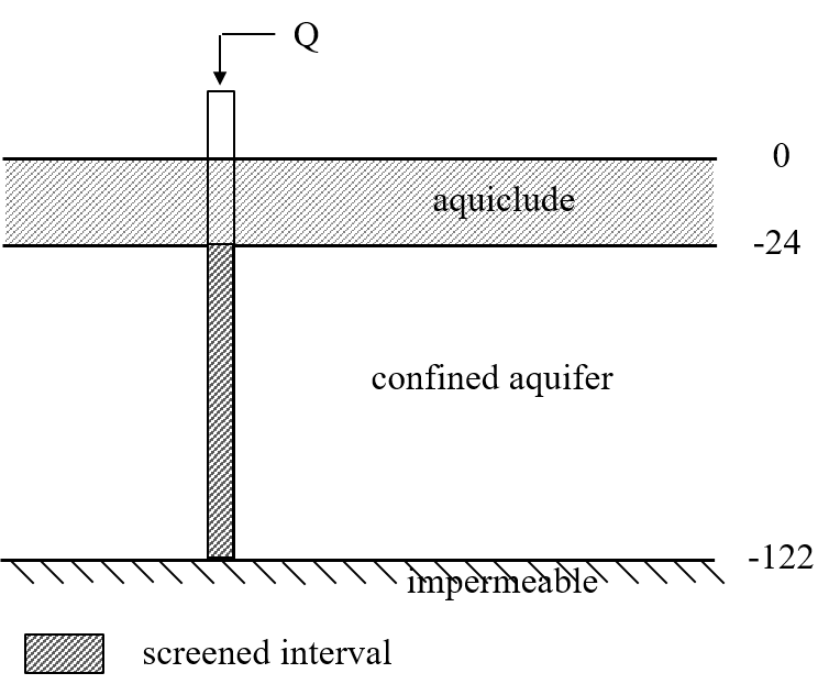
A fully penetrated well (Ln-2) is screened in a confined aquifer, located between depths 24 and 122 (98 m thick). The volume of the slug is 10.16 litres. Head change has been recorded at the slug well. Both the well and the casing radii of the slug well is 0.076 m.
Load data#
data = np.loadtxt("data/dawsonville_slug.txt")
to = data[:, 0]
ho = data[:, 1]
Parameters and model#
# known parameters
b = 98  # aquifer thickness in m
zt = -24  # top of aquifer in m
zb = zt - b  # bottom of aquifer in m
rw = 0.076  # well radius of Ln-2 Well in m
rc = 0.076  # casing radius of Ln-2 Well in m
Q = 10.16 / 1000  # slug volume in m^3 (10.16 l = 0.01016 m^3)
ml = tft.ModelMaq(kaq=10, z=[zt, zb], Saq=1e-4, tmin=1e-6, tmax=1e-3, topboundary="conf")
w = tft.Well(ml, xw=0, yw=0, rw=rw, rc=rc, tsandQ=[(0, -Q)], layers=0, wbstype="slug")
ml.solve()
self.neq  1
solution complete
Estimate aquifer parameters#
We calibrate hydraulic conductivity and specific storage, as in the KGS model (Hyder et al. 1994).
# unknown parameters: kay, Saq
cal = tft.Calibrate(ml)
cal.set_parameter(name="kaq0", initial=10, pmin=0, layers=0)
cal.set_parameter(name="Saq0", initial=1e-4, layers=0)
cal.seriesinwell(name="obs", element=w, t=to, h=ho)
cal.fit(report=False)
...............................
Fit succeeded.
display(cal.parameters)
print("rmse:", cal.rmse())
| layers | optimal | std | perc_std | pmin | pmax | initial | inhoms | parray | |
|---|---|---|---|---|---|---|---|---|---|
| kaq0_0_0 | 0 | 0.420908 | 0.018325 | 4.353689 | 0.0 | inf | 10.0000 | None | [[0.42090788883700814]] |
| Saq0_0_0 | 0 | 0.000017 | 0.000005 | 31.025816 | -inf | inf | 0.0001 | None | [[1.7004312750679313e-05]] |
rmse: 0.004409616694582213
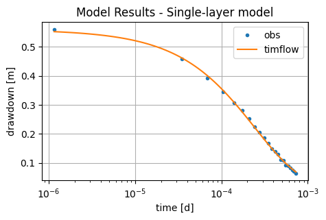
tm = np.logspace(np.log10(to[0]), np.log10(to[-1]), 100)
hm = ml.head(0, 0, tm)
plt.semilogx(to, ho, ".", label="obs")
plt.semilogx(tm, hm[0], label="timflow")
plt.xlabel("time [d]")
plt.ylabel("drawdown [m]")
plt.title("Model Results - Single-layer model")
plt.legend()
plt.grid()
Comparison of results#
We now compare the values in timflow and add the results of the modelling done in MLU (Hemker & Post, 2014). Results are similar between both models. The RMSE of MLU is slightly better than the one from timflow.
| k [m/d] | Ss [1/m] | RMSE [m] | |
|---|---|---|---|
| timflow | 0.42 | 1.70e-05 | 0.004 |
| MLU | 0.41 | 1.94e-05 | 0.004 |
References#
Cooper Jr, H.H., Bredehoeft, J.D. and Papadopulos, I.S. (1967) Response of a finite diameter well to an instantaneous charge of water, Water Resources Research 3, 263–269
Duffield, G.M. (2007), AQTESOLV for Windows Version 4.5 User’s Guide, HydroSOLVE, Inc., Reston, VA.
Hemker, K. en Post V. (2014) MLU for Windows: well flow modeling in multilayer aquifer systems; MLU User’s guide. https://eur03.safelinks.protection.outlook.com/?url=https%3A%2F%2Fmicrofem.com%2Fdownload%2Fmlu-user.pdf&data=05%7C02%7CMark.Bakker%40tudelft.nl%7Cad7f16364d2d4fd55dbf08de73832eaa%7C096e524d692940308cd38ab42de0887b%7C0%7C0%7C639075204580287861%7CUnknown%7CTWFpbGZsb3d8eyJFbXB0eU1hcGkiOnRydWUsIlYiOiIwLjAuMDAwMCIsIlAiOiJXaW4zMiIsIkFOIjoiTWFpbCIsIldUIjoyfQ%3D%3D%7C0%7C%7C%7C&sdata=OBoe8seXZUfoat89Dfr4g6lF%2Bn1FdtXqtp%2F18BMXCn0%3D&reserved=0
Hyder, Z., Butler Jr, J.J., McElwee, C.D. and Liu, W. (1994) Slug tests in partially penetrating wells, Water Resources Research 30, 2945–2957.