2. Confined Aquifer Test - Gridley

Import packages

import matplotlib.pyplot as plt
import numpy as np
import pandas as pd

import timflow.transient as tft

plt.rcParams["figure.figsize"] = (5, 3)  # default figure size

Introduction and Conceptual Model

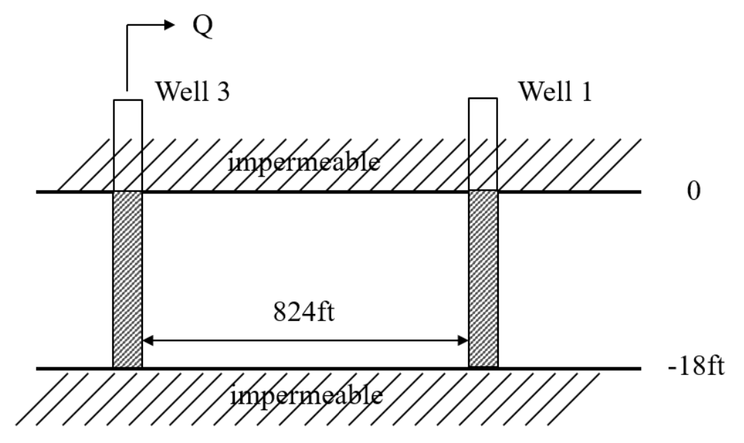
This example is a pumping test conducted in 1953 in Gridley, Illinois, US. It was reported by Walton (1962).

The aquifer is an 18 ft thick sand and gravel layer under confined conditions. The pumping well fully penetrates the formation, and pumping was conducted for 8 hours at a rate of 220 gallons per minute. The effect of pumping was observed at observation well 1, located 824 ft away from the well.

The time-drawdown data for the observation well were obtained from the AQTESOLV documentation (Duffield, 2007), while data from the pumping well were obtained from the original paper from Walton (1962). Following AQTESOLV documentation (Duffield, 2007), radii of 0.5 ft were used for both the pumping and observation wells.

Load data

# Loading Observation well (Well 1)
data1 = np.loadtxt("data/gridley_well_1.txt")
to1 = data1[:, 0]
ho1 = data1[:, 1]

# Loading Pumping Well data (Well 3)
data2 = np.loadtxt("data/gridley_well_3.txt")
to2 = data2[:, 0]
ho2 = data2[:, 1]

Parameters and model

# known parameters
H = 18 * 0.3048  # aquifer thickness in m (18 ft = 5.48 m)
Q = (
    (220 * 0.00378541) * 60 * 24
)  # constant discharge in m^3/d (220 gallons/minute = 1199.22 m^3/d)
r = (
    824 * 0.3048
)  # distance between observation well to test well in m (824 ft = 251.16 m)
rw = 0.5 * 0.3048  # screen radius of test well in m (0.5 ft = 0.15 m)

Wellbore storage is added to the model.

ml = tft.ModelMaq(kaq=10, z=[0, -H], Saq=0.001, tmin=0.001, tmax=1, topboundary="conf")
w = tft.Well(ml, xw=0, yw=0, rw=rw, tsandQ=[(0, Q)], rc=rw, layers=0)
ml.solve()

self.neq  1
solution complete

Estimate aquifer parameters

The aquifer parameters are estimated using both datasets simultaneously.

# unknown parameters: kaq, Saq
cal = tft.Calibrate(ml)  # create Calibrate object
cal.set_parameter(
    name="kaq", initial=10, layers=0
)  # setting the parameters for calibration
cal.set_parameter(name="Saq", initial=1e-4, pmin=1e-7, layers=0)
cal.series(name="obs1", x=r, y=0, t=to1, h=ho1, layer=0)  # setting the observation data
cal.seriesinwell(name="obs2", element=w, t=to2, h=ho2)  # setting the observation data
cal.fit(report=False)

............................
Fit succeeded.

display(cal.parameters.loc[:, ["optimal"]])
print(f"RMSE: {cal.rmse():.3f} m")

	optimal
kaq_0_0	38.086506
Saq_0_0	0.000001

RMSE: 0.259 m

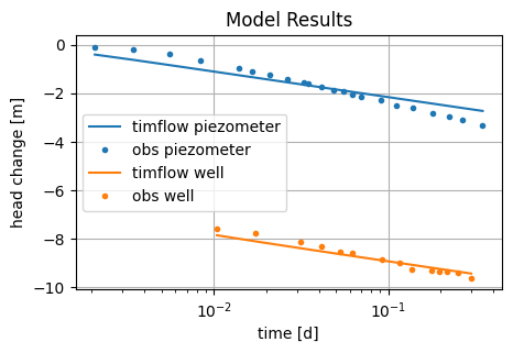
hm1 = ml.head(r, 0, to1)
hm2 = w.headinside(to2)
plt.semilogx(to1, hm1[0], "C0", label="timflow piezometer")
plt.semilogx(to1, ho1, "C0.", label="obs piezometer")
plt.semilogx(to2, hm2[0], "C1", label="timflow well")
plt.semilogx(to2, ho2, "C1.", label="obs well")
plt.title("Model Results")
plt.xlabel("time [d]")
plt.ylabel("head change [m]")
plt.legend()
plt.grid()

Comparison of results

The performance of timflow is compared to the results based on Theis’ analytical solution (Theis, 1935), implemented in the software AQTESOLV (Duffield, 2007).

Results from timflow with added wellbore storage differ largely from those from AQTESOLV. This difference is due to the missing wellborage storage in the AQTESOLV model.

Show code cell source

Hide code cell source

t = pd.DataFrame(
    columns=["k [m/d]", "Ss [1/m]", "RMSE [m]"], index=["timflow", "AQTESOLV"]
)

t.loc["timflow"] = np.append(cal.parameters["optimal"].values, cal.rmse())
t.loc["AQTESOLV"] = [22.95, 0.000003722, "-"]

t_formatted = t.style.format(
    {
        "k [m/d]": "{:.2f}",
        "Ss [1/m]": "{:.2e}",
        "RMSE [m]": lambda x: "-" if x == "-" else f"{float(x):.3f}",
    }
)
t_formatted

	k [m/d]	Ss [1/m]	RMSE [m]
timflow	38.09	1.19e-06	0.259
AQTESOLV	22.95	3.72e-06	-

References

• Duffield, G.M. (2007), AQTESOLV for Windows Version 4.5 User’s Guide, HydroSOLVE, Inc., Reston, VA.

• Walton, W.C. (1962), Selected analytical methods for well and aquifer evaluation, Illinois, department of Registration & Education.bulletin 49.