4. Confined Aquifer Test - Nevada#
Import packages#
import matplotlib.pyplot as plt
import numpy as np
import pandas as pd

import timflow.transient as tft

plt.rcParams["figure.figsize"] = (5, 3)  # default figure size
Introduction and Conceptual Model#
This example is taken from Kruseman and de Ridder (1990). It is based on a pumping test conducted in a fractured tertiary volcanic aquifer near Yucca Mountains, Nevada, US.
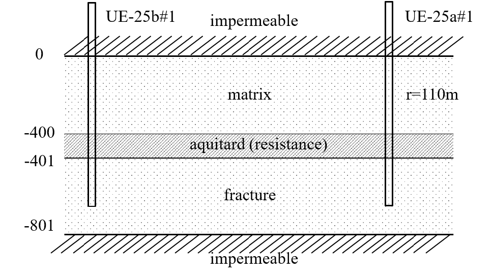
The borehole extends to 1219 m depth and penetrates a 400 m thick sequence of fractured volcanic rocks with water entry points. At every entry point, the head is more or less the same, so they have good hydraulic connection. The water table is about 470 m below land surface, which indicates confined conditions. Drawdown data was monitored at the well, named UE-25b#1 and at an observation well, named UE-25a#1, 110 m away. Three pumping tests were conducted at the site and will be the object of our investigation.
Although conventional Darcy flow does not apply to flow in discrete fractures, the fracture network at this site is sufficiently pervasive to justify the application of Darcy’s law at the aquifer scale. Groundwater flow to the well occurs through fractures, while the matrix exchanges water with the fracture network. For implementation in timflow, the fractured aquifer system is approximated using a ModelMaq configuration. This is achieved by representing the matrix as an upper aquifer layer, separated by a 1 m thick aquitard from a lower aquifer layer representing the fracture network.
Load Data#
# time and drawdown of pumped well UE-25b#1
data1 = np.loadtxt("data/double-porosity-pumpingwell.txt", skiprows=1)
t1 = data1[:, 0]  # days
h1 = data1[:, 1]  # m

# time and drawdown of observation well UE-25a#1
data2 = np.loadtxt("data/double-porosity-110m.txt", skiprows=1)
t2 = data2[:, 0]
h2 = data2[:, 1]
Paramaters and model#
# known parameters
H = 400  # aquifer thickness in m
Q = 3093.12  # constant pumping rate in m^3/d
r = 110  # distance from pumping well to observation well in m
For the timflow model, we will adopt the parameters for the first layer from the results obtained from Kruseman and de Ridder (1970).
# parameters calculated by Kruseman and de Ridder (1970)
km = 0.1 / H  # hydraulic conductivity of matrix
Sm = 3.75e-4  # specific storage of matrix
ml = tft.ModelMaq(
    kaq=[km, 1],
    z=[0, -400, -401, -801],
    c=5,
    Saq=[Sm, 1e-3],
    Sll=0,
    topboundary="conf",
    tmin=1e-5,
    tmax=3,
)
w = tft.Well(ml, xw=0, yw=0, rw=0.11, rc=0, tsandQ=[0, Q], layers=1)
ml.solve()
self.neq  1
solution complete
Estimate aquifer parameters#
The aquifer parameters are estimated using head observations at both wells.
cal = tft.Calibrate(ml)
cal.set_parameter(name="kaq", initial=10, layers=1)
cal.set_parameter(name="Saq", initial=1e-4, pmin=0, layers=1)
cal.set_parameter(name="c", initial=10, layers=1)
cal.set_parameter_by_reference(name="rc", parameter=w.rc, initial=0)

cal.seriesinwell(name="UE-25b#1", element=w, t=t1, h=h1)
cal.series(name="UE-25a#1", x=r, y=0, t=t2, h=h2, layer=1)
cal.fit(report=False)
..................
...................
...................
...................
...................
...................
...................
...................
...................
...................
.............
Fit succeeded.
display(cal.parameters.loc[:, ["optimal"]])
print(f"RMSE: {cal.rmse():.3f} m")
| optimal | |
|---|---|
| kaq_1_1 | 0.877139 |
| Saq_1_1 | 0.000005 |
| c_1_1 | 12.912907 |
| rc | 0.105678 |
RMSE: 0.198 m
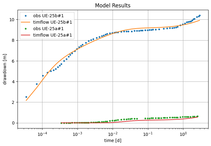
hm1 = w.headinside(t1)
hm2 = ml.head(r, 0, t2)
plt.figure(figsize=(8, 5))
plt.semilogx(t1, -h1, ".", label="obs UE-25b#1")
plt.semilogx(t1, -hm1[-1], label="timflow UE-25b#1")
plt.semilogx(t2, -h2, ".", label="obs UE-25a#1")
plt.semilogx(t2, -hm2[-1], label="timflow UE-25a#1")
plt.xlabel("time [d]")
plt.ylabel("drawdown [m]")
plt.title("Model Results")
plt.legend()
plt.grid();
Comparison of results#
The performance of timflow was evaluated by comparison to the results obtained from the software AQTESOLV (Duffield, 2007), MLU (Hemker & Post, 2014), and Kruseman and de Ridder (1990), here abbreviated to K&dR.
The problem is solved in AQTESOLV using a double-porosity analytical solution proposed by Moench (1984). The MLU (Hemker & Post, 2014) solution used a similar approach to our timflow model by simulating the matrix as a very-low transmissivity aquifer on top of the fractured aquifer and separated by a zero-storage aquitard. However, the calibrated MLU model only fits the observations of well UE-25b#1. When the observations of well UE-25a#1 are included, the fit is not as good as initially thought. Kruseman et al. (1990) solved the problem using a graphical method, where the transmissivity was calculated as one aquifer and the storativity was separated between matrix and fractures.
Overall, timflow showed similar results to MLU but with a better fit since both observation wells are taken into account with the timflow model. While the AQTESOLV obtained the best fit using Moench’s analytical solution.
| km [m/d] | Sm [1/m] | kf [m/d] | Sf [1/m] | c [d] | rc [m] | RMSE [m] | |
|---|---|---|---|---|---|---|---|
| timflow | 0.00 | 3.75e-04 | 0.88 | 5.07e-06 | 12.91 | 0.11 | 0.198 |
| AQTESOLV | 0.15 | 5.48e-04 | 0.94 | 1.95e-03 | - | 0.11 | - |
| MLU | 0.00 | 3.75e-04 | 0.84 | 8.05e-06 | 5.20 | - | - |
| K&dR | 0.83 | 3.75e-04 | 0.83 | 4.00e-06 | - | - | - |
Reference#
Duffield, G.M. (2007), AQTESOLV for Windows Version 4.5 User’s Guide, HydroSOLVE, Inc., Reston, VA.
Hemker, K. en Post V. (2014) MLU for Windows: well flow modeling in multilayer aquifer systems; MLU User’s guide. https://eur03.safelinks.protection.outlook.com/?url=https%3A%2F%2Fmicrofem.com%2Fdownload%2Fmlu-user.pdf&data=05%7C02%7CMark.Bakker%40tudelft.nl%7Cad7f16364d2d4fd55dbf08de73832eaa%7C096e524d692940308cd38ab42de0887b%7C0%7C0%7C639075204580287861%7CUnknown%7CTWFpbGZsb3d8eyJFbXB0eU1hcGkiOnRydWUsIlYiOiIwLjAuMDAwMCIsIlAiOiJXaW4zMiIsIkFOIjoiTWFpbCIsIldUIjoyfQ%3D%3D%7C0%7C%7C%7C&sdata=OBoe8seXZUfoat89Dfr4g6lF%2Bn1FdtXqtp%2F18BMXCn0%3D&reserved=0
Kruseman, G.P. and De Ridder, N.A. (1990), Analysis and evaluation of pumping test data, 2nd edn. ILRI Publ. 47, ILRI, Wageningen, The Netherlands
Moench, A.F. (1984), Double-Porosity Models for a Fissured Groundwater Reservoir With Fracture Skin, Water Resour. Res., 20( 7), 831– 846, doi:10.1029/WR020i007p00831.