3. Slug Test - Falling Head

Import packages

import matplotlib.pyplot as plt
import numpy as np
import pandas as pd

import timflow.transient as tft

plt.rcParams["figure.figsize"] = [5, 3]

Introduction and Conceptual Model

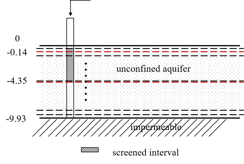
A well partially penetrates a sandy unconfined aquifer that has a saturated depth of 32.57 ft. The top of the screen is located 0.47 ft below the water table and has 13.8 ft in length. The well and casing radii are 5 and 2 inches, respectively. The slug displacement is 1.48 ft. Head change has been recorded at the slug well. This slug test, taken from the AQTESOLV examples (Duffield, 2007), was reported in Batu (1998).

Load data

data = np.loadtxt("data/falling_head.txt", skiprows=2)
to = data[:, 0] / 60 / 60 / 24  # convert time from seconds to days
ho = (10 - data[:, 1]) * 0.3048  # convert drawdown from ft to meters

Parameters and model

rw = 5 * 0.0254  # well radius, m
rc = 2 * 0.0254  # well casing radius, m
L = 13.8 * 0.3048  # screen length, m
b = 32.57 * 0.3048  # aquifer thickness, m
zt = 0  # top of aquifer, m
zst = -0.47 * 0.3048  # top of screen, m
zsb = zst - L  # bottom of screen, m
zb = zt - b  # bottom of aquifer, m
H0 = 1.48 * 0.3048  # initial displacement in well, m

convert measured displacement into volume

Q = np.pi * rc**2 * H0
print(f"slug: {Q:.5f} m^3")

slug: 0.00366 m^3

We will create a multi-layer model. For this, we divide the second and third layers into 0.5 m thick layers.

# z = np.array([zt, zt - 0.1, zst, zsb, zb])
z = np.hstack(
    (
        zt,
        np.linspace(zt - 0.01, zst, 5)[:-1],
        np.linspace(zst, zsb, 5)[:-1],
        np.linspace(zsb, zb, 10),
    )
)
nlay = len(z) - 1
nlay

18

z

array([ 0.      , -0.01    , -0.043314, -0.076628, -0.109942, -0.143256,
       -1.194816, -2.246376, -3.297936, -4.349496, -4.969256, -5.589016,
       -6.208776, -6.828536, -7.448296, -8.068056, -8.687816, -9.307576,
       -9.927336])

ml = tft.Model3D(
    kaq=10,
    z=z,
    Saq=[0.1] + (nlay - 1) * [1e-4],
    kzoverkh=1,
    tmin=1e-5,
    tmax=0.01,
    phreatictop=True,
)
w = tft.Well(
    ml,
    xw=0,
    yw=0,
    rw=rw,
    tsandQ=[(0, -Q)],
    layers=range(6, 6 + 5),
    rc=rc,
    wbstype="slug",
)
ml.solve()

self.neq  5
solution complete

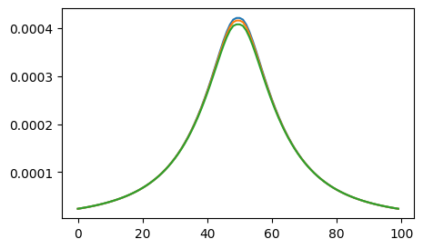
r = np.linspace(-10, 10, 100)
h = ml.headalongline(r, 0, 0.01).squeeze()
plt.plot(h[0])
plt.plot(h[1])
plt.plot(h[2])

[<matplotlib.lines.Line2D at 0x7959db320e10>]

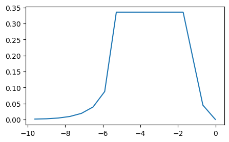
t = np.logspace(-5, -2, 100)
h = ml.head(0, 0, t)
zc = 0.5 * (z[:-1] + z[1:])
plt.plot(zc, h[:, 10])

[<matplotlib.lines.Line2D at 0x7959db3c7d90>]

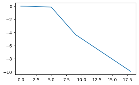
plt.plot(z)

[<matplotlib.lines.Line2D at 0x7959db24b4d0>]

Estimate aquifer parameters

cal = tft.Calibrate(ml)
cal.set_parameter(name="kaq", layers=list(range(1, nlay)), initial=10, pmin=0)
cal.set_parameter(name="Saq", layers=list(range(1, nlay)), initial=1e-4, pmin=0)
cal.seriesinwell(name="obs", element=w, t=to, h=ho)
cal.fit(report=False)

..............
..............
.......
Fit succeeded.

display(cal.parameters.loc[:, ["optimal"]])
print(f"RMSE: {cal.rmse():.3f} m")

	optimal
kaq_1_17	0.439175
Saq_1_17	0.000461

RMSE: 0.006 m

tm = np.logspace(np.log10(to[0]), np.log10(to[-1]), 100)
hm = w.headinside(tm)
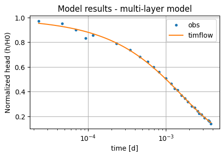
plt.semilogx(to, ho / H0, ".", label="obs")
plt.semilogx(tm, hm[0] / H0, label="timflow")
plt.xlabel("time [d]")
plt.ylabel("Normalized head (h/H0)")
plt.title("Model results - multi-layer model")
plt.legend()
plt.grid()

Comparison of results

Here, the timflow performance in analysing slug tests is checked. The solution in timflow is compared with the KGS analytical model (Hyder et al. 1994) implemented in AQTESOLV (Duffield, 2007). The parameters of timflow and AQTESOLV are similar, even though AQTESOLV only used one layer.

Show code cell source

Hide code cell source

t = pd.DataFrame(
    columns=["k [m/d]", "Ss [1/m]", "RMSE [m]"],
    index=["timflow", "AQTESOLV"],
)

t.loc["timflow"] = np.append(cal.parameters["optimal"].values, cal.rmse())
t.loc["AQTESOLV"] = [0.4211, 5.70e-4, "-"]

t_formatted = t.style.format(
    {
        "k [m/d]": "{:.2f}",
        "Ss [1/m]": "{:.2e}",
        "RMSE [m]": lambda x: "-" if x == "-" else f"{float(x):.3f}",
    }
)
t_formatted

	k [m/d]	Ss [1/m]	RMSE [m]
timflow	0.44	4.61e-04	0.006
AQTESOLV	0.42	5.70e-04	-

References

• Batu, V. (1998), Aquifer hydraulics: a comprehensive guide to hydrogeologic data analysis, John Wiley & Sons

• Duffield, G.M. (2007), AQTESOLV for Windows Version 4.5 User’s Guide, HydroSOLVE, Inc., Reston, VA.

• Hyder, Z., Butler Jr, J.J., McElwee, C.D. and Liu, W. (1994), Slug tests in partially penetrating wells, Water Resources Research 30, 2945–2957.